Let’s start with some definitions:
A hypothesis is a function that maps an input from the entire input space to a result: \(h:\mathcal{X}\to\{-1,+1\}\) The number of hypotheses $\vert\mathcal{H}\vert$ can be infinite.
A dichotomy is a hypothesis that maps from an input from the sample size to a result:
\[h:\{\mathbf{x}_1,\mathbf{x}_2,\dots,\mathbf{x}_N\}\to\{-1,+1\}\]The number of dichotomies $\vert\mathcal{H}(\mathbf{x}_1,\mathbf{x}_2,\dots,\mathbf{x}_N )\vert$ is at most $2^N$, where $N$ is the sample size.
e.g. for a sample size $N = 3$ we have at most $8$ possible dichotomies:
1
2
3
4
5
6
7
8
9
10
        x1 x2 x3
1	-1 -1 -1
2	-1 -1 +1
3	-1 +1 -1
4	-1 +1 +1
5	+1 -1 -1
6	+1 -1 +1
7	+1 +1 -1
8	+1 +1 +1
The growth function is a function that counts the most dichotomies on any $N$ points. \(m_{\mathcal{H}}(N)=\underset{\mathbf{x}_1,\dots,\mathbf{x}_N\in\mathcal{X}}{max}\vert\mathcal{H}(\mathbf{x}_1,\dots,\mathbf{x}_N)\vert\) This translates into choosing any $N$ points and laying them out in any fashion in the input space. Determining $m$ is equivalent to looking for such a layout of the $N$ points that yields the most dichotomies.
The growth function satisfies: \(m_{\mathcal{H}}(N)\le 2^N\) This can be applied to the perceptron. For example, when $N=4$, we can lay out the points so that they are easily separated. However, given a layout, we must then consider all possible configurations of labels on the points, one of which is the following:
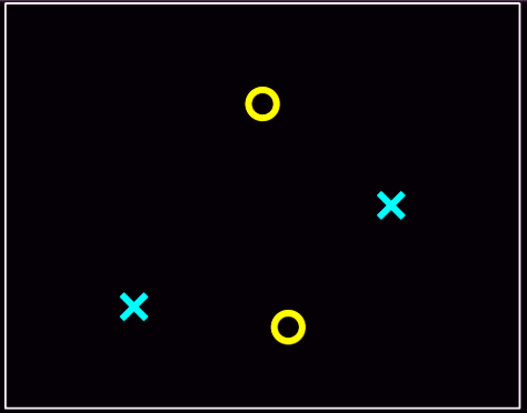
This is where the perceptron breaks down because it cannot separate that configuration, and so $m_{\mathcal{H}}(4)=14$ because two configurations—this one and the one in which the left/right points are blue and top/bottom are red—cannot be represented. For this reason, we have to expect that for perceptrons, $m$ can’t be $2^4$.
The VC ( Vapnik-Chervonenkis ) dimension of a hypothesis set $\mathcal{H}$ , denoted by $d_{VC}(\mathcal{H})$ is the largest value of $N$ for which $m_{\mathcal{H}}(N)=2^N$ , in other words is “the most points $\mathcal{H}$ can shatter “
We can say that the VC dimension is one of many measures that characterize the expressive power, or capacity, of a hypothesis class.
You can think of the VC dimension as “how many points can this model class memorize/shatter?” (a ton? $\to$ BAD! not so many? $\to$ GOOD!).
With respect to learning, the effect of the VC dimension is that if the VC dimension is finite, then the hypothesis will generalize:
\[d_{vc}(\mathcal H)\ \Longrightarrow\ g \in \mathcal H \text { will generalize }\]The key observation here is that this statement is independent of:
- The learning algorithm
- The input distribution
- The target function
The only things that factor into this are the training examples, the hypothesis set, and the final hypothesis.
The VC dimension for a linear classifier (i.e. a line in 2D, a plane in 3D etc…) is $d+1$ (a line can shatter at most $2+1=3$ points, a plane can shatter at most $3+1=4$ points etc…)
Proof: here
How many randomly drawn examples suffice to guarantee error of at most $\epsilon$ with probability at least (1−$\delta$)?
\[N\ge\frac{1}{\epsilon}\left(4\log\left(\frac{2}{\delta}\right)+8VC(H)\log_2\left(\frac{13}{\epsilon}\right)\right)\]PAC BOUND using VC dimension:
\[L_{true}(h)\le L_{train}(h)+\sqrt{\frac{VC(H)\left(\ln\frac{2N}{VC(H)}+1\right)+\ln\frac{4}{\delta}}{N}}\]